Clocks and Causality - Ordering Events in Distributed Systems

Share this article

Introduction

System events could be arranged in an order based on the time they occurred. Clocks keep time and produce timestamps. Conventional clocks (such as time-of-day clocks) use a common reference to learn time. That reference could be internal hardware or a common service that serves time using protocols like NTP. However, because of clock drifts and/or assumptions around network time delays, timestamps from conventional clocks are not always mutually comparable, and therefore events cannot be reliably ordered using timestamps from conventional clocks.

A logical clock is a custom clock that is designed to produce timestamps that can be reliably compared. (We will see shortly that timestamps from logical clocks take a different form than the timestamps from time-of-day clocks). If multiple nodes in a distributed system can rely on a centralized logical clock, then most issues discussed in this article become irrelevant. However, a centralized clock by definition is neither fault-tolerant nor can offer performance beyond a limit. In this article, therefore, we are primarily interested in distributed logical clocks spread across multiple nodes.

For a distributed logical clock to function, we expect each of the participating nodes to have its own clock that cooperates with clocks on other nodes in order to produce the next timestamp. When dealing with distributed logical clocks, we are primarily interested in the time of occurrence of system events on any node so that we could order such events across nodes according to their timestamps.

Events cannot obviously consider the effects of future events. However, because events may occur faster than the notification of such events between nodes, events may be unaware of some past events. Events that occur without the knowledge of each other are called concurrent events. Events, at best, can be ordered according to their originating timestamps in real-time only when there are no concurrent events. That is, none of the logical clocks discussed in this article help with ordering events in real-time in the presence of concurrent events. That said, not all clocks can order events even in the absence of concurrent events. This article discusses why such clocks are still useful.

The article will also demonstrate that in non-real-time (i.e., after the fact), we can arrange events in a total order using some clocks. Total order means if each of the nodes have a collection of events, then all nodes can individually arrive at the same order of events. Total order respects happened-before (and causality) relationships. The Event Ordering section at the end of this article discusses total order in detail.

Clock Designs

The various logical clock designs we will study in this article essentially implement a variation of the following solution:

Each timestamp produced by a logical clock consists of two components:

1. an id for the current event, and
2. the ids of some or all events the node is aware of thus far (aka history).

Tracking all historical events in a timestamp is space consuming. Richness in the timestamp therefore needs to be purchased with space or time complexity. And different designs make different choices in this area. However, a common compaction scheme used by different clock designs is to track history with the use of numbers for event ids. Under this compaction scheme, an event with timestamp [ 5 ] not only represents that the event id is the number 5, but that the node generating that event has knowledge of the existence of (some) event [ 4 ] (because there could be multiple [ 4 ] events) and possibly all events prior to and equal to [ 4 ], depending on the clock.

Note that causality and history (i.e., happened-before events) are related concepts, but not identical. If the knowledge from event A is used to produce event B, then A caused B. If B merely happened before C, but event C did not use the knowledge from event B, then B and C are not causally related, just temporally so. Most applications, for simplicity, use temporal relationship as a proxy for causality.

Let us look at various logical clock designs.

Lamport Clock

Timestamps produced by a Lamport clock take the least amount of space, O(1) in terms of the number of nodes in the system, compared to other clock designs. A Lamport timestamp captures the event id and some history of events the node is aware of at the time the event is generated, all using a single unique number. When a node generated event id [ 5 ], the node claims to have knowledge of some event that is numbered [ 4 ] and no knowledge of any other event that is numbered [ 5 ] or above.

Lamport timestamps do not capture which node generated the event. Therefore, there might be events with the same timestamps from different nodes circulating in the system. Consequently, looking at the timestamps of two events, say [ 4 ] and [ 5 ], one cannot answer whether event [ 5 ] is aware of that particular event [ 4 ] or a different event [ 4 ]. Overall, given that event [ 4 ] has knowledge of some event [ 3 ], and [ 3 ] of some [ 2 ], and so on, it is understood that event [ 5 ] has knowledge of the existence of some events [ 4 ] through [ 1 ].

A Lamport clock can be implemented as follows:

1. Timestamps are sequential numbers associated with events.
2. Each node maintains its own sequence starting with number 0.
3. When an event is generated, the node increments its number by one and associates that number with the event.
4. When a node learns an event from another node, the node ensures its number to be the highest of its own number and the event number it learned from the other node.
   • In this article, we consider a learning event as any other event, and have the node increment its number by one.
   • Some applications do not timestamp learning events.

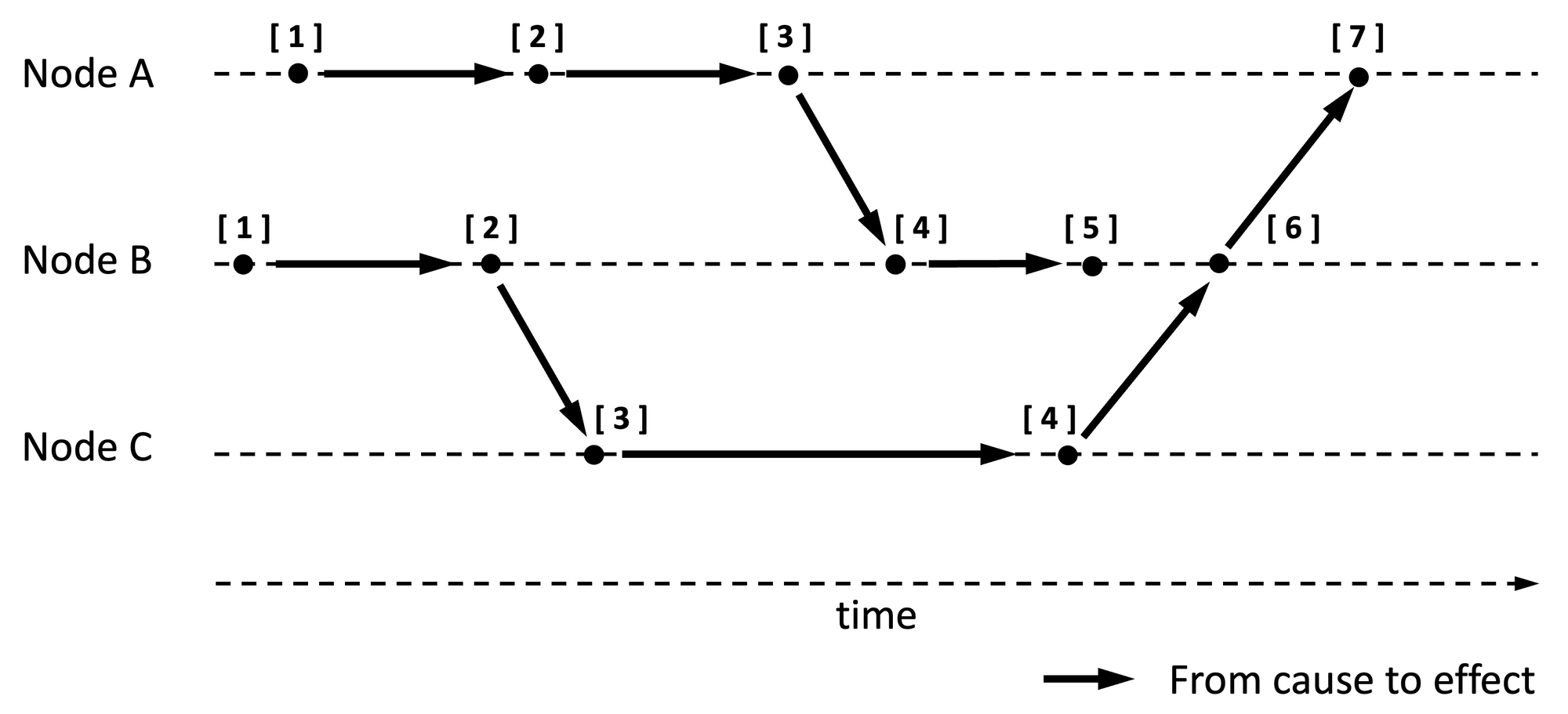
Overall, Lamport timestamps are strictly increasing numbers in any given node, and at least monotonically increasing across nodes. See Figure 1 for an illustration. Arrows are pointed at effects by causes.

Why are Lamport timestamps useful? Lamport timestamps can be used to arrange events in a historical (i.e., happened-before) order after the fact. Specifically,

1. Events across nodes can be ordered in a way that also honors local order: Because each timestamp produced by a node is a strictly increasing number, when events are ordered based on timestamps, all local events of a node will retain their order of generation even when events from other nodes are in the mix.
2. Events can be arranged based on history (aka happened-before): While there are duplicate event timestamps across nodes, when events are arranged in an increasing order based on timestamps, an event with the knowledge of another event will always follow it in the order (because the event id reflects a higher number than the ids of the events it is aware of).
3. Events can be causal ordered: Causes are by definition known events; therefore, causal ordering follows from 2 above.

Lamport clocks have three deficiencies:

• A total order of events is not deterministically possible with Lamport timestamps. Events have duplicate timestamps, e.g., multiple events with id [ 4 ], and those events cannot be ordered in any deterministic way.
• While events can be arranged in a way that honors historical and causal ordering, you can only do so after the fact, but not in real-time. A node may know about or have generated event [ 5 ] first and then learned about event [ 4 ] some time later. As a result, if order preservation while processing non-concurrent events in real-time is important, Lamport clock is not adequate.
• Relatedly, it is not evident from Lamport timestamps if an event definitely occurred after another event or if the two events are concurrent. For example, in Figure 1, it is not clear if event [ 5 ] is an effect of event [ 4 ] produced on node B or event [ 4 ] produced on node C.

Lamport Origin Clock

A variant of Lamport Clock, hereafter referred to as Lamport Origin Clock, can produce a timestamp that is a doublet consisting of [node id, Lamport timestamp]. Lamport origin timestamp can be used to arrange events after the fact in a predictable order using originating node id as the second sort property. This removes the first deficiency of Lamport clocks discussed above, but it does not remove the other deficiencies of not knowing the order in real-time even for non-concurrent events.

Figure 2 is an update of Figure 1 with origin information included in the timestamp.

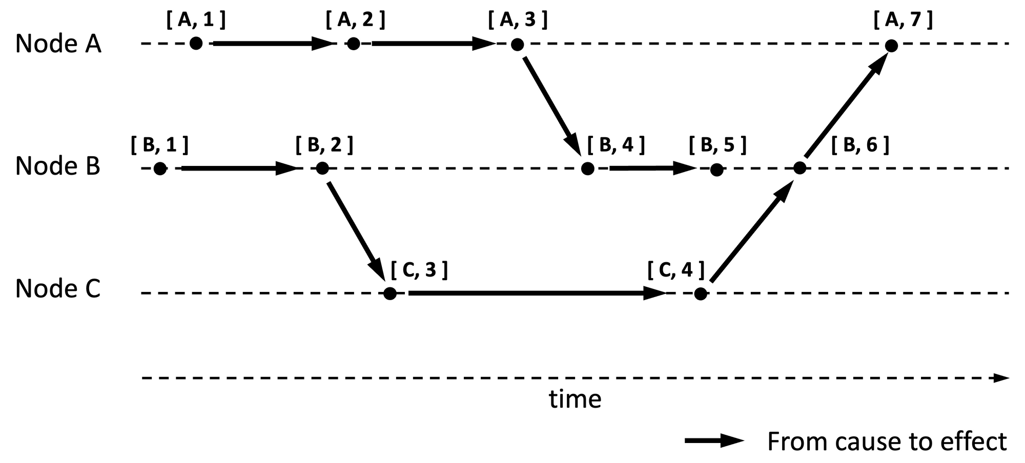
Lamport origin timestamp can also be used as a unique identifier for events because the  combination of node id and Lamport timestamp is unique across events from any node. The space complexity is still O(1).

We will look at one last variation of Lamport clock after we review vector clocks.

Vector Clock and Dotted Vector Clock

Timestamps produced by a vector clock take the most amount of space compared to other well-known clock designs. The space complexity is O(n). A vector timestamp tracks the id of a node and the last known event id from that node. Therefore, if there are n nodes in the system, the timestamp would be an n-tuple.

The number compaction scheme applies here too, but in a slightly richer way than in Lamport clocks. Here, if node A knows of event [ 5 ] from node B, then node A knows of the existence of events [ 1 ] through [ 5 ] from node B.

Let us learn the characteristics of a vector timestamp from an example. See Figure 3 for a companion illustration.

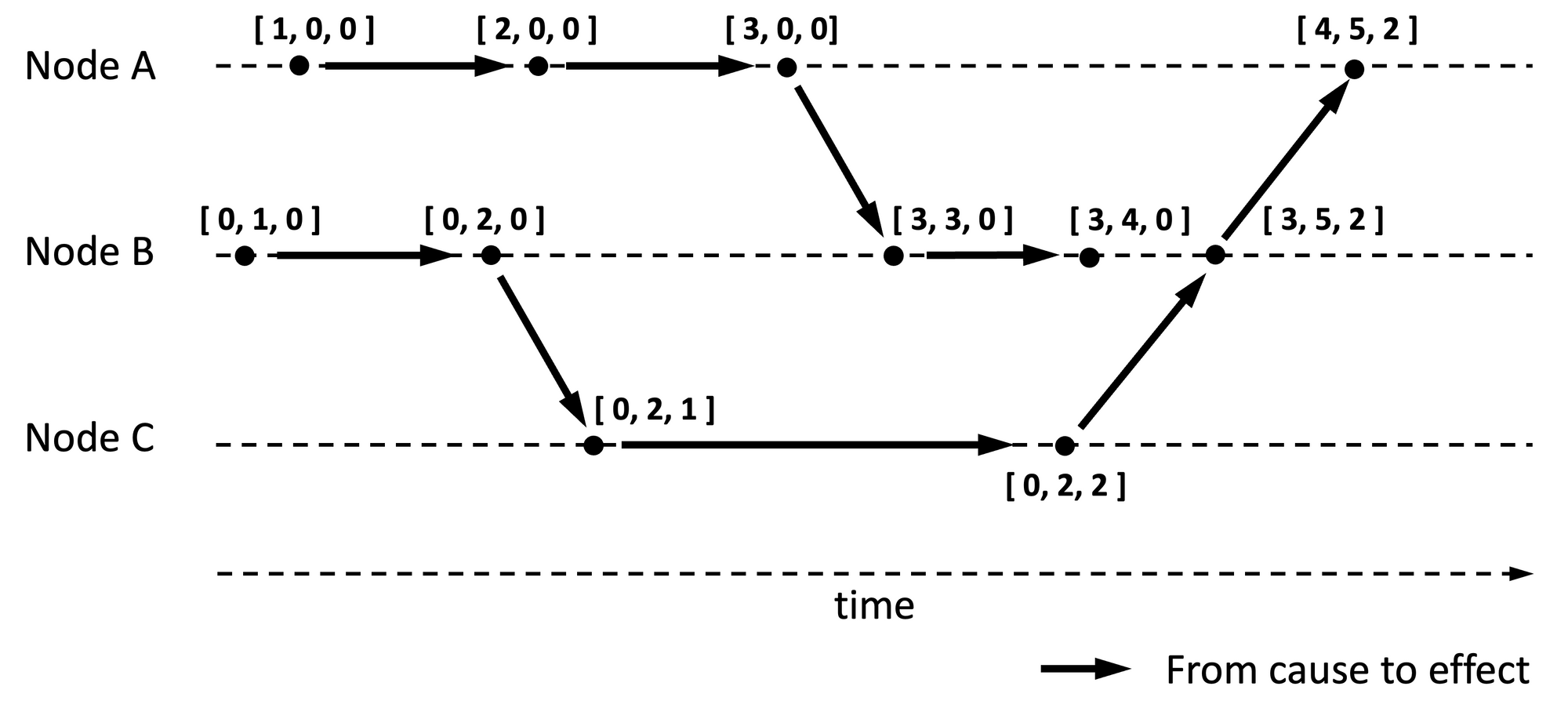
If say [3, 4, 0] is a vector timestamp associated with an event on node B, then the timestamp is conveying:

• There are overall three nodes in this distributed system because the timestamp is a triplet.
• This event is the fourth event generated by node B, as indicated by the number 4 in the triplet.
• At the time when node B generated this event, it is aware of the existence of the first three events generated by node A and none of the events from node C.
• It precedes events like [4, 5, 2] because event [4, 5, 2] would have been aware of the existence of all events implied in [3, 4, 0].
• It is concurrent with event [0, 2, 2] because event [ 2 ] on node C happened without the knowledge of event [ 4 ] (or [ 3 ]) on node B (and vice versa). See comparison algorithm below.

Vector timestamps can be compared as follows. Compare each entry from one n-tuple timestamp with the corresponding entry in another n-tuple timestamp.

• If all entries are identical, then the timestamps are the same, e.g., [3, 4, 0] against [3, 4, 0].
• If some entries are less or equal, and some entries are greater, the timestamps are concurrent, e.g., [3, 4, 0] and [0, 2, 2]. The greater entries are in bold.
• If one or more entries are less and none are greater, the timestamp with lower entry values precedes the other timestamp, e.g., [3, 4, 0] precedes [4, 5, 2].

The comparison time complexity is O(n) as there are n entries to compare before deciding the ordinality of two events. Comparisons can be reduced to O(1) if the last event is separately tracked in the vector timestamp. Since vector timestamps keep track of the history of events from every node (via compaction), timestamp T1 will have been issued before another timestamp T2 if the last event of T1 is part of T2. No other checks need to be made to determine the order. Generally speaking, the algorithm is to check if the last event of one timestamp is part of another. If neither, then the timestamps are concurrent.

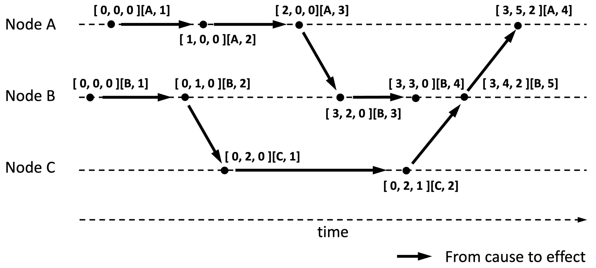
Dotted Vector Clock takes advantage of this optimization. The term dot refers to the last occurring event. Dotted vector clock tracks the latest event as a dot (in bold) separately, like so: [3, 3, 0][B, 4]. Here, event [ 4 ] on node B is the latest event. In a conventional vector timestamp format [3, 3, 0][B, 4] would be equivalent to [3, 4, 0].

Given two dotted timestamps, [3, 3, 0][B, 4] and [3, 5, 2][A, 4], it is easy to observe [B, 4] dot from the first timestamp is encapsulated within the second timestamp by checking against the entry for the B node in the tuple, which is 5, and therefore infer that the first timestamp precedes the second timestamp without any further checks. It might be necessary to check the dot from one timestamp with the dot from another timestamp, in case the timestamps are the same.

Figure 4 is an update of Figure 3 with vector timestamps represented in dotted form.

A vector clock can be implemented as follows:

1. Each node maintains its own sequence starting with number 0.
2. Nodes never mix sequence numbers from other nodes, unlike Lamport timestamps. Nodes maintain sequence numbers associated with each node in that node’s portion of the n-tuple.
3. When an event is generated, the node increments its number by one and associates that number with the event.
4. When an event from another node is observed, the node keeps track of the latest event from that node in the portion of the n-tuple that is designated for that node. That is, there is one entry per node.
   • In this article, we consider a learning event as any other event, and have the learning node increment its own number by one.
5. In the case of a dotted vector clock, instead of performing the steps in 3 or 4, the last event either generated by the node or as observed from another node is captured in a dot. A dot is a doublet [node id, number]. node id is the generator of the last event. number is the latest sequence observed from that node. The previous dot is enrolled into the n-tuple by incrementing the number associated with the node indicated in the dot.

Why are vector timestamps useful? Since they carry a superset of information compared to Lamport origin timestamps, they have the same advantages as Lamport origin timestamps and more:

1. Events across nodes can be ordered in a way that also honors local order. Events can also be ordered based on history (and therefore implicitly based on causality). Ordering of non-concurrent events can happen in real-time, unlike the two Lamport clock variants we discussed above, because knowledge of the existence of preceding events is encoded in a vector timestamp.
2. Events can be uniquely identified across nodes.
3. Vector timestamps can be used to designate an event to have succeeded multiple concurrent events; essentially, a merge of different branches of concurrent events stemming from another event. For example, the event [3, 5, 2] on node B could be considered the effect of two concurrent events: [3, 4, 0] on node B and [0, 2, 2] on node C. Encoding this information is not possible with Lamport clock variants because they use a single number across nodes. This attribute of vector clocks is useful in scenarios where a merge of data from different branches is made and the event timestamp should signify the merge of multiple branches of data.

Note, however, that vector timestamps do not explicitly capture causality. They capture history. Lamport causal clock discussed below captures causality explicitly and has almost the same properties as vector clock.

Version Vector and Dotted Version Vector

A version vector is not a clock in its own right, but a use case of vector clocks. However, I discuss this topic in this article because version vectors are incorrectly used interchangeably with vector clocks by some articles.

Version vectors are a clever use of vector clocks, and are typically employed by multi-leader storage nodes to track versions of stored data (and not events). Storage nodes use version vectors as follows:

1. A vector clock is maintained by storage nodes as before, but timestamps are issued only when data is modified (which results in a new version of data). Specifically, timestamps are used to denote versions of data. Hence the word version in its name.
2. Each data item that needs to be tracked for changes will have its own vector clock.
3. The number of nodes in the timestamp tuple reflect the number of leader storage nodes that make changes to data. For example, if there are three leaders, the timestamp would be a triple, with each segment reflecting changes made by each of the leaders. The implication is that clients that contribute to data changes are not tracked in the timestamp tuple (because there could be a large number of clients). The space complexity of version vectors is therefore O(n), where n is the number of leader storage nodes.
4. Clients follow the read, update, and write pattern: a client reads data from a storage node along with the vector timestamp (aka version) of the data read; the client updates data and sends the update to the storage node along with the timestamp it read.
5. If the storage node’s current timestamp matches the timestamp sent by the client, that is if there are no changes to data since the client last read, the storage node simply increments the timestamp/version of the updated data and stores it.
6. If the node’s current timestamp is different from what the client sent, then there are concurrent changes made to data. The storage node increments the timestamp, like in case 4, and associates that timestamp with the data version. However, the node preserves the previous version of data (and its timestamp) and awaits manual resolution of data divergence. When the conflict is manually resolved, a single future timestamp is associated with the converged data.
7. When data changes on a storage node are replicated to other storage nodes, the receiving nodes either accept the changes and converge data or keep track of changes separately depending on whether the changes received are succeeding changes or concurrent changes, just like in points (5) and (6) above.

If a vector clock used in the version vector is dotted, then the version vector is considered a dotted version vector.

Let us now revert to our clocks discussion.

Lamport Causal Clock

The space complexity of a vector timestamp is O(n). To reduce the space complexity, some applications use Lamport timestamps or Lamport origin timestamps, which both have a space complexity of O(1). However, as we observed above, Lamport timestamp variants have inferior functionality compared to vector timestamps. To recall, one drawback of Lamport timestamps is that we cannot deduce if an event definitely occurred after another event or if they are definitely concurrent. Vector timestamps can.

To address this deficiency while still keeping the space complexity of timestamps to O(1) (although with a few more constant number of bits added), some applications add the causal event timestamp to the Lamport origin timestamp.

This variant of Lamport clock, hereafter referred to as Lamport Causal Clock, has a few characteristics, which we will study using the example of an event with timestamp [A, 7, [B, 6] ]:

• It is event [ 7 ] generated by node A. [ 7 ] and [A, 7] would be its conventional Lamport timestamp and Lamport origin timestamp respectively.
• It is caused by event [ 6 ] generated on node B.

Figure 5 illustrates events with causal information included in the timestamp.

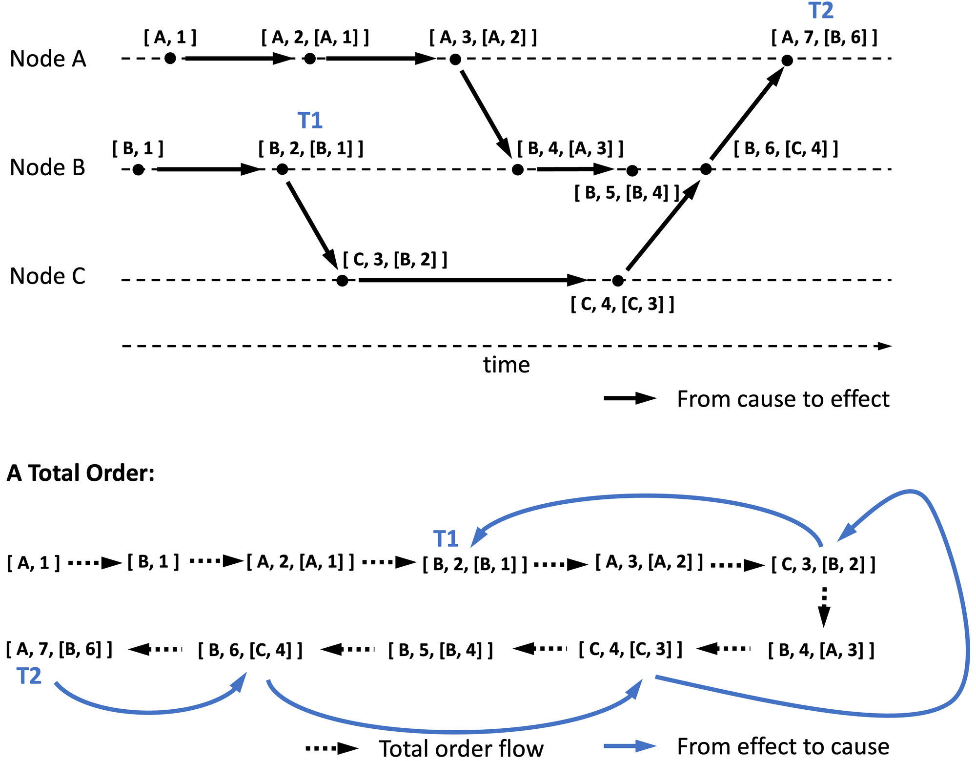
Unlike any other clocks we have seen so far, Lamport causal clock explicitly captures the causal event. Recall that vector clocks capture history, not causality specifically. We will see how this knowledge can be used to order events in the next section on Event Ordering.

To compare two Lamport causal timestamps, say T1 and T2, when there are m events total, the following procedure can be used.

1. If T1 and T2 are the same, then the corresponding events are the same. Comparison stops here. Otherwise, proceed.
2. Identify the timestamp with the highest Lamport timestamp, e.g., the first timestamp amongst [A, 7, [B, 6] ] and [B, 2, [B, 1] ] because [ 7 ] is higher than  [ 2 ]. (Recall that Lamport timestamps synchronize sequences between nodes). Let us call the higher of the two events T2 and the other event T1. It is evident that T2 occurred either later than T1 or concurrently with T1.
3. Order the known events from the beginning until T2. Recall that we can use Lamport origin timestamps to order known events after the fact. The time complexity of this step itself is O(m log m), (a typical sort algorithm based on event numbers and node ids). This step may not be needed if you can trivially recall events needed for step 4 and 5 below.
   
   Figure 5 illustrates the ordered events at the bottom, with black (not blue) arrows indicating the resulting order once this step is followed. You may not know yet, but this results in a total order of events (next section discusses this topic).
4. Track back from T2 towards the beginning following the causal events. For example the causal event for T2 is [B, 6]. Its causal event can be found in the timestamp associated with it in the ordered list, and so on.
5. Repeat step 4 until either T1 is found or an event with a lower Lamport timestamp than T1 (or the beginning) is found. This has O(m) time complexity. If skip lists are used, then the time complexity could be reduced to O(log m).
6. If T1 is found, then T1 is in the causal chain of T2. Therefore T2 succeeds T1. In Figure 5, the blue arrows indicate the flow of events from effects to causes, forming a path from T2 to T1.
7. If T1 is not found in the causal chain, but a lower Lamport origin timestamp than T1 is found or the beginning is reached, then T1 is concurrent with T2.

As you can observe, the vector clock functionality can be achieved with a Lamport causal clock and with less space complexity, O(1) vs O(n). However, dotted vector timestamps allow you to compare two events in O(1) time complexity compared to O(log m) with Lamport causal timestamps, after events are either ordered or can be trivially recalled. Otherwise the time complexity will go up to O(m log m) primarily due to step 3 above.

Event Ordering

We have passingly observed how timestamps from various logical clocks can be used to order system events. Let us explicitly study one desirable order for many applications: Total Order.

Total Order (TO)

For an event order to be considered a TO, two conditions have to be met:

1. Causes must precede effects. That is, events that cause other events should precede in the order. (Recall that some systems use temporally preceding events as causes, which is fine).
2. Concurrent events must be ordered the same way by different nodes when those events are learned.

Why is the first condition important? Since we generally create systems that can deal with events in real-time, we prefer an order that honors temporal and causal relationships. The first rule essentially ensures events that are meant to be processed sequentially are not scattered arbitrarily in the final order.

Why is the second condition important? Readers familiar with graph models will have known topological sorting. Topological sorting is the sorting of vertices of a directed acyclic graph where vertex u appears before vertex v in the final order if there is an edge from u to v. Depending on the graph, there could be multiple orders that honor topological sorting rules, and this is the crux of the issue that the second condition observes.

In our case, there are edges from causes to effects, and topological sorting will order events where causes appear before effects (condition 1 above). The problem is that the presence of concurrent events will result in multiple ordering possibilities. Our goal is to have a predictable order that each node can arrive at while processing events. The second condition is essentially a stipulation to guarantee that predictability.

One way to achieve TO is as follows:

• Assume the first event is a null event, and use the null event as the cause for events with no causes.
• Causes precede effects. That is, effects should follow causes in the order.
• When multiple events have the same cause, position those events after the cause using Lamport timestamp in the decreasing order, where (latter) events with higher numbers are positioned first. A variant of this is to position earlier events first.
• If there are two events with the same event number, arrange events in the increasing order of the event origins (i.e., node ids).

See Figure 6 for an example. I refer to the TO ordering resulting from the above rules as CTO, for easier reference.

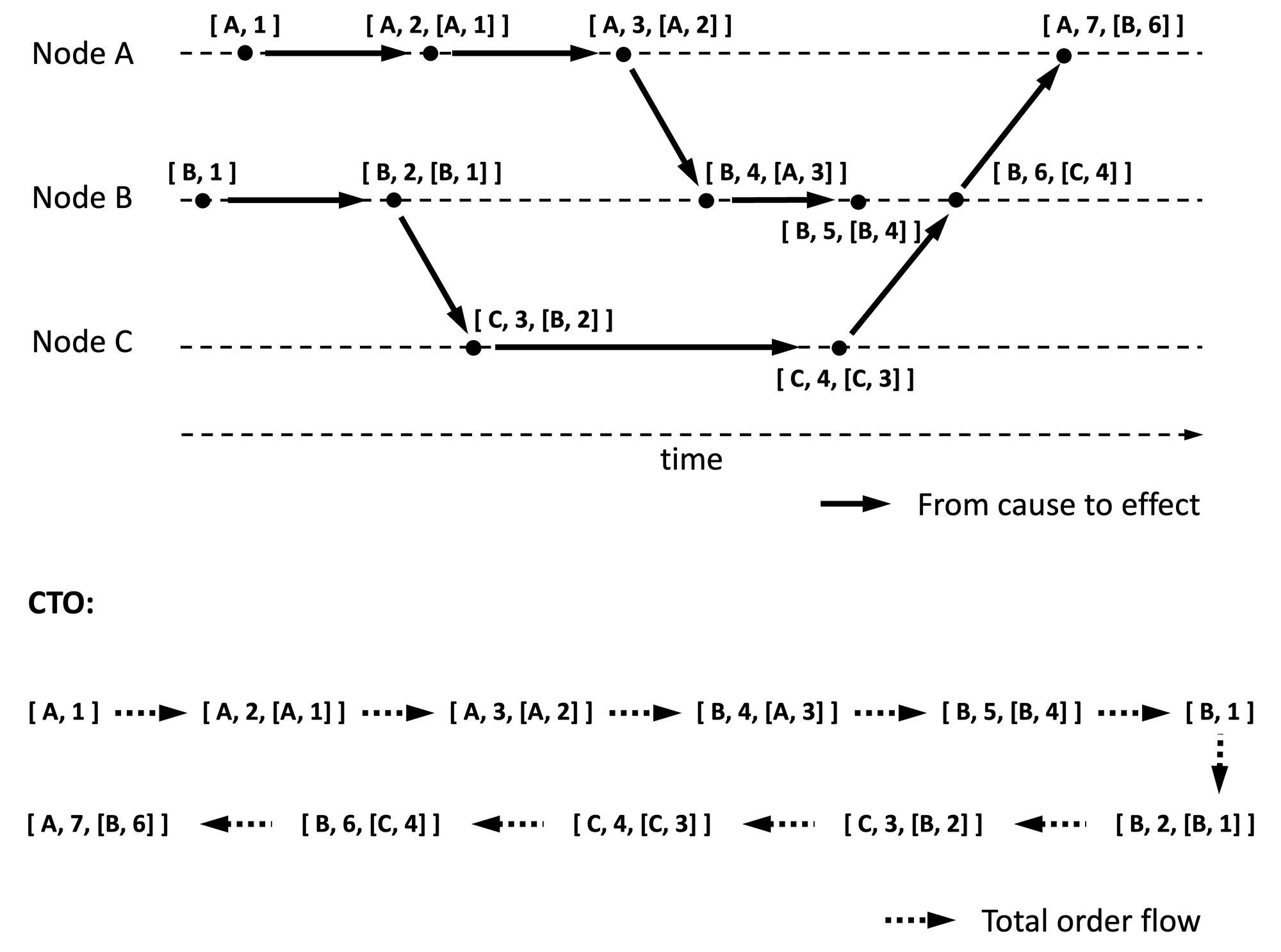
The idea behind CTO is that if events are replayed as defined here, then causes are processed before effects (which is the natural order) and when there are competing effects to causes, a sub-algorithm is chosen based on the situation, as explained next.

When competing effects are from multiple nodes, then effects are arranged using the node ordering (i.e., based on node id). Because of choosing node id arbitrarily to break the tie, this ordering is sometimes referred to as arbitrary total order. When competing effects are from the same node, the recent effects are given precedence for arriving at the total order. A variation of this is when the oldest among the competing effects are given precedence instead of the recent ones. Which variation is useful depends on whether the most recent competing effect should override prior effects or add to the outcome.

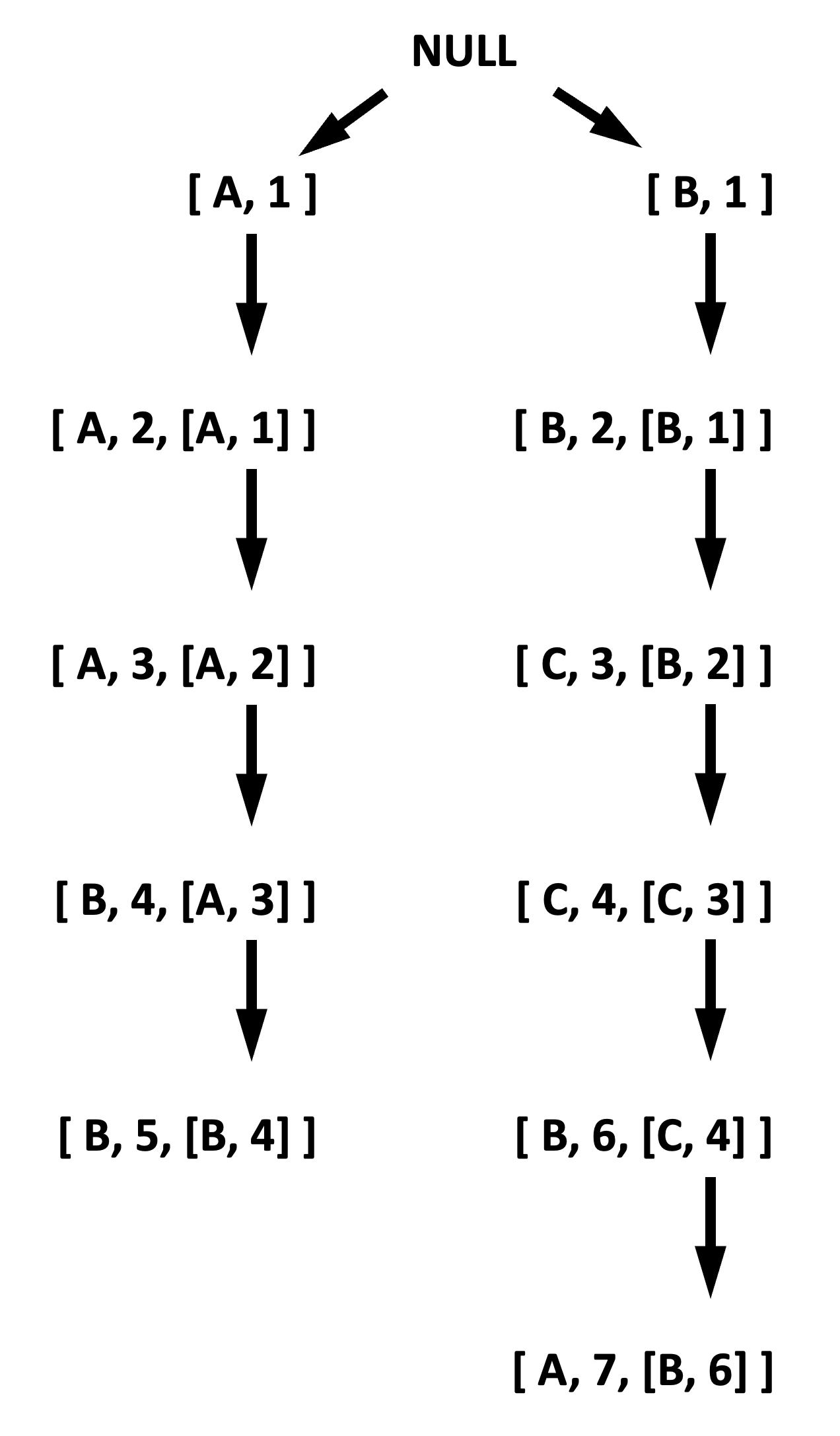
It turns out that either of these CTO variations can be produced by performing a preorder depth-first traversal of a mythical tree of events where every root of a subtree is the cause and children are the effects. That tree is referred to in literature as Causal Tree. A causal tree of events from Figure 6 are illustrated in Figure 7.

Why is CTO style of TO important? Some collaborative-editing applications rely on this event order for arriving at the same text when multiple users are simultaneously producing events that mutate the text (an offline-supported Google docs of sort).

We could arrive at other forms of TO besides CTO. For example, the ordering performed in step 3 in the timestamp comparison algorithm for Lamport causal clock described above results in a TO. Why? The ordering is based on Lamport timestamps. And as we noted in the Lamport clock section, we could arrive at a causal order using Lamport timestamps after the fact. This meets condition 1 for TO. When we have concurrent events, we used node ids to break the ties when running the comparison algorithm. And node ids based sorting is deterministic, meeting condition 2 for TO. (We could also arrive at this particular TO using vector timestamps instead of Lamport causal timestamps because the extra knowledge of causality embedded in Lamport causal clock is ignored in this TO). Let us refer to this TO as NCTO, for reference.

Clocks and Event Ordering

Event orderings that can be produced under various clock designs. Some characteristics of the produced event orders are stated below.

• None of the clocks discussed in this article can be used to achieve total order in real-time because of the presence of concurrent events. However, some clocks can achieve total order in real-time when there are no ongoing concurrent events.
• Lamport Clock (LC) cannot be used to achieve total order in real-time even amongst non-concurrent events. However, after the fact, events when arranged in ascending order of event numbers, the resulting order conforms to historical (and therefore causal) order, but not total order. That is, the order is indeterministic because of the presence of duplicate event numbers (i.e., no criteria can be applied to consider one duplicate before other). One other limitation is that the order cannot indicate whether two events are concurrent events or one is an effect of another.
• Lamport Origin Clock (LOC) cannot be used to achieve total order in real time even amongst non-concurrent events and the relationship between two events cannot be determined, which are the same limitations as LC. However, after the fact, events can be arranged in total order (that agrees with historical and causal order). The node id can be used as a second sort property to deal with duplicate event numbers.
• Both LC and LOC are not preferable options for some event-replay dependent applications because ordering is only possible after the fact.
• Vector Clock (VC) can be used to achieve total order after the fact, or in real-time barring concurrent events. Such an order would be in NCTO form.
• Lamport Causal Clock (LCC), like VC, can be used to achieve total order after the fact, or in real-time barring concurrent events. And the ordering could be in NCTO form or in CTO because LCC tracks causal events. But producing a total order with LCC is slower in practice compared to with VC. LCC is space efficient, however.

Given m events, LC and LOC can be used to order with a time complexity of O(m log m), as any two events can be compared to determine which events come first, and the problem therefore reduces to sorting m elements. VC can also be used to order events with a time complexity of O(m log m) because each timestamp consists of the entire history, thereby, again, reducing the problem to sorting m elements. The assumption is that a dotted vector clock is used, so that comparing two timestamps will be O(1) in terms of the number of nodes.

LCC can be used to order events with a time complexity of O(m log m) similar to timestamps from other clock designs. But skip lists should be maintained to achieve that complexity. With a naive implementation, the time complexity will be O(m²). The increase in complexity compared to other timestamps is because two timestamps produced by LCC cannot just be mutually compared to infer the order; historical events should also be consulted that requires a traversal back. In other words, comparing any two LCC timestamps without skip lists has a time complexity of O(m).

Conclusion

Conventional clocks have safety issues. Centralized clocks have liveness and performance issues. Logical clocks solve those issues, and are therefore used by many distributed systems, especially storage systems. Multi-leader storage systems use logical clocks for conflict resolution. Leaderless storage systems use them for repairs and anti-entropy mechanisms. Conflict-free replicated data types (CRDTs), which are cooperating data structures that can mutate data while being disconnected from each other, use logical clocks as their foundation to preemptively deal with conflicts.

Given the foundational role logical clocks play in the design of distributed systems, it is only fitting to learn about them. This article discussed the internals of various logical clock designs and the tradeoffs we have to make in choosing one design over the other.

---